Tim DiPalo

import pandas as pd
from statsmodels.formula.api import ols as sm_ols
import numpy as np
import seaborn as sns
from statsmodels.iolib.summary2 import summary_col # nicer tables

Part 1: EDA

Insert cells as needed below to write a short EDA/data section that summarizes the data for someone who has never opened it before.

Answer essential questions about the dataset (observation units, time period, sample size, many of the questions above)
Note any issues you have with the data (variable X has problem Y that needs to get addressed before using it in regressions or a prediction model because Z)
Present any visual results you think are interesting or important

housing = pd.read_csv('input_data2/housing_train.csv')
housing

	parcel	v_MS_SubClass	v_MS_Zoning	v_Lot_Frontage	v_Lot_Area	v_Street	v_Alley	v_Lot_Shape	v_Land_Contour	v_Utilities	...	v_Pool_Area	v_Pool_QC	v_Fence	v_Misc_Feature	v_Misc_Val	v_Mo_Sold	v_Yr_Sold	v_Sale_Type	v_Sale_Condition	v_SalePrice
0	1056_528110080	20	RL	107.0	13891	Pave	NaN	Reg	Lvl	AllPub	...	0	NaN	NaN	NaN	0	1	2008	New	Partial	372402
1	1055_528108150	20	RL	98.0	12704	Pave	NaN	Reg	Lvl	AllPub	...	0	NaN	NaN	NaN	0	1	2008	New	Partial	317500
2	1053_528104050	20	RL	114.0	14803	Pave	NaN	Reg	Lvl	AllPub	...	0	NaN	NaN	NaN	0	6	2008	New	Partial	385000
3	2213_909275160	20	RL	126.0	13108	Pave	NaN	IR2	HLS	AllPub	...	0	NaN	NaN	NaN	0	6	2007	WD	Normal	153500
4	1051_528102030	20	RL	96.0	12444	Pave	NaN	Reg	Lvl	AllPub	...	0	NaN	NaN	NaN	0	11	2008	New	Partial	394617
...	...	...	...	...	...	...	...	...	...	...	...	...	...	...	...	...	...	...	...	...	...
1936	2524_534125210	190	RL	79.0	13110	Pave	NaN	IR1	Lvl	AllPub	...	0	NaN	MnPrv	NaN	0	7	2006	WD	Normal	146500
1937	2846_909131125	190	RH	NaN	7082	Pave	NaN	Reg	Lvl	AllPub	...	0	NaN	NaN	NaN	0	7	2006	WD	Normal	160000
1938	2605_535382020	190	RL	60.0	10800	Pave	NaN	Reg	Lvl	AllPub	...	0	NaN	NaN	NaN	0	5	2006	ConLD	Normal	160000
1939	1516_909101180	190	RL	55.0	5687	Pave	Grvl	Reg	Bnk	AllPub	...	0	NaN	NaN	NaN	0	3	2008	WD	Normal	135900
1940	1387_905200100	190	RL	60.0	12900	Pave	NaN	Reg	Lvl	AllPub	...	0	NaN	NaN	NaN	0	1	2008	WD	Alloca	95541

1941 rows × 81 columns

Essential Questions:

The unit of observation is a house/property

The time period is the years 2006 to 2008, with a fairly even distribution of observations between those years

The parcel variable is a unique identifier for this dataset

The dataset has a sample size of 1941 observations

Many of the variables in this dataset are categorical, mostly describing different types of property or of certain features. For example:

v_MS_Zoning: Identifies the general zoning classification of the sale.
v_MS_SubClass: Identifies the type of dwelling involved in the sale
v_Neighborhood: Physical locations within Ames city limits

Some variables in the dataset are continuous or discrete, with many showing the square footage of certain features of the property. For example:

v_Lot_Area: Lot size in square feet
v_Low_Qual_Fin_SF: Low quality finished square feet (all floors)
v_Fireplaces: Number of fireplaces

Potential Issues

Some variables have large amounts of missing data, however I believe these often just indicate a property that doesn’t have whatever that variable is talking about. For example, v_Fence has 1,576 missing values, but when looking at the documentation, it is clear that properties without a fence are filled with NaN values

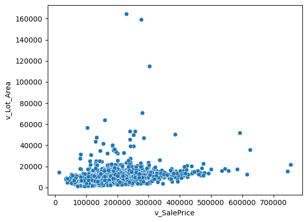
I was able to identify some outliers using scatterplots for v_SalePrice with one of the variables we will be using in the regressions, v_Lot_Area. This plot can be seen below.

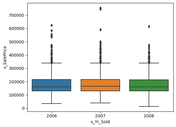
The box plot showing the sales price by years also displays these outliers above the maximum sale price. This plot can be seen below

sns.scatterplot(x='v_SalePrice', y='v_Lot_Area', data=housing)

<AxesSubplot: xlabel='v_SalePrice', ylabel='v_Lot_Area'>

png

sns.boxplot(x='v_Yr_Sold', y='v_SalePrice', data=housing)

<AxesSubplot: xlabel='v_Yr_Sold', ylabel='v_SalePrice'>

png

Data Visualization Takeaways

Continuous variables: Sales price and Lot Area - Seen above, this relationship seems linear, with some outliers

Categorical variables: Sales price and Year Sold - Seen above, this relationship also shows outliers in the sales price

Part 2: Running Regressions

Run these regressions on the RAW data, even if you found data issues that you think should be addressed.

Insert cells as needed below to run these regressions. Note that $i$ is indexing a given house, and $t$ indexes the year of sale.

$\text{Sale Price}_{i,t} = \alpha + \beta_1 * \text{v_Lot_Area}$
$\text{Sale Price}_{i,t} = \alpha + \beta_1 * log(\text{v_Lot_Area})$
$log(\text{Sale Price}_{i,t}) = \alpha + \beta_1 * \text{v_Lot_Area}$
$log(\text{Sale Price}_{i,t}) = \alpha + \beta_1 * log(\text{v_Lot_Area})$
$log(\text{Sale Price}_{i,t}) = \alpha + \beta_1 * \text{v_Yr_Sold}$
$log(\text{Sale Price}_{i,t}) = \alpha + \beta_1 * (\text{v_Yr_Sold==2007})+ \beta_2 * (\text{v_Yr_Sold==2008})$
Choose your own adventure: Pick any five variables from the dataset that you think will generate good R2. Use them in a regression of $log(\text{Sale Price}_{i,t})$
- Tip: You can transform/create these five variables however you want, even if it creates extra variables. For example: I’d count Model 6 above as only using one variable: v_Yr_Sold.
- I got an R2 of 0.877 with just “5” variables. How close can you get? I won’t be shocked if someone beats that!

Bonus formatting trick: Instead of reporting all regressions separately, report all seven regressions in a single table using summary_col.

reg1 = sm_ols(
    "v_SalePrice ~ v_Lot_Area", data=housing
).fit()
reg1.summary()

OLS Regression Results
Dep. Variable:	v_SalePrice	R-squared:	0.067
Model:	OLS	Adj. R-squared:	0.066
Method:	Least Squares	F-statistic:	138.3
Date:	Sun, 02 Apr 2023	Prob (F-statistic):	6.82e-31
Time:	16:13:19	Log-Likelihood:	-24610.
No. Observations:	1941	AIC:	4.922e+04
Df Residuals:	1939	BIC:	4.924e+04
Df Model:	1
Covariance Type:	nonrobust

	coef	std err	t	P>\|t\|	[0.025	0.975]
Intercept	1.548e+05	2911.591	53.163	0.000	1.49e+05	1.6e+05
v_Lot_Area	2.6489	0.225	11.760	0.000	2.207	3.091

Omnibus:	668.513	Durbin-Watson:	1.064
Prob(Omnibus):	0.000	Jarque-Bera (JB):	3001.894
Skew:	1.595	Prob(JB):	0.00
Kurtosis:	8.191	Cond. No.	2.13e+04

Notes:
[1] Standard Errors assume that the covariance matrix of the errors is correctly specified.
[2] The condition number is large, 2.13e+04. This might indicate that there are
strong multicollinearity or other numerical problems.

reg2 = sm_ols(
    "v_SalePrice ~ np.log(v_Lot_Area)", data=housing
).fit()
reg2.summary()

OLS Regression Results
Dep. Variable:	v_SalePrice	R-squared:	0.128
Model:	OLS	Adj. R-squared:	0.128
Method:	Least Squares	F-statistic:	285.6
Date:	Sun, 02 Apr 2023	Prob (F-statistic):	6.95e-60
Time:	16:13:19	Log-Likelihood:	-24544.
No. Observations:	1941	AIC:	4.909e+04
Df Residuals:	1939	BIC:	4.910e+04
Df Model:	1
Covariance Type:	nonrobust

	coef	std err	t	P>\|t\|	[0.025	0.975]
Intercept	-3.279e+05	3.02e+04	-10.850	0.000	-3.87e+05	-2.69e+05
np.log(v_Lot_Area)	5.603e+04	3315.139	16.901	0.000	4.95e+04	6.25e+04

Omnibus:	650.067	Durbin-Watson:	1.042
Prob(Omnibus):	0.000	Jarque-Bera (JB):	2623.687
Skew:	1.587	Prob(JB):	0.00
Kurtosis:	7.729	Cond. No.	164.

Notes:
[1] Standard Errors assume that the covariance matrix of the errors is correctly specified.

reg3 = sm_ols(
    "np.log(v_SalePrice) ~ v_Lot_Area", data=housing
).fit()
reg3.summary()

OLS Regression Results
Dep. Variable:	np.log(v_SalePrice)	R-squared:	0.065
Model:	OLS	Adj. R-squared:	0.064
Method:	Least Squares	F-statistic:	133.9
Date:	Sun, 02 Apr 2023	Prob (F-statistic):	5.46e-30
Time:	16:13:19	Log-Likelihood:	-927.19
No. Observations:	1941	AIC:	1858.
Df Residuals:	1939	BIC:	1870.
Df Model:	1
Covariance Type:	nonrobust

	coef	std err	t	P>\|t\|	[0.025	0.975]
Intercept	11.8941	0.015	813.211	0.000	11.865	11.923
v_Lot_Area	1.309e-05	1.13e-06	11.571	0.000	1.09e-05	1.53e-05

Omnibus:	75.460	Durbin-Watson:	0.980
Prob(Omnibus):	0.000	Jarque-Bera (JB):	218.556
Skew:	-0.066	Prob(JB):	3.48e-48
Kurtosis:	4.639	Cond. No.	2.13e+04

reg4 = sm_ols(
    "np.log(v_SalePrice) ~ np.log(v_Lot_Area)", data=housing
).fit()
reg4.summary()

OLS Regression Results
Dep. Variable:	np.log(v_SalePrice)	R-squared:	0.135
Model:	OLS	Adj. R-squared:	0.135
Method:	Least Squares	F-statistic:	302.5
Date:	Sun, 02 Apr 2023	Prob (F-statistic):	4.38e-63
Time:	16:13:19	Log-Likelihood:	-851.27
No. Observations:	1941	AIC:	1707.
Df Residuals:	1939	BIC:	1718.
Df Model:	1
Covariance Type:	nonrobust

	coef	std err	t	P>\|t\|	[0.025	0.975]
Intercept	9.4051	0.151	62.253	0.000	9.109	9.701
np.log(v_Lot_Area)	0.2883	0.017	17.394	0.000	0.256	0.321

Omnibus:	84.067	Durbin-Watson:	0.955
Prob(Omnibus):	0.000	Jarque-Bera (JB):	255.283
Skew:	-0.100	Prob(JB):	3.68e-56
Kurtosis:	4.765	Cond. No.	164.

Notes:
[1] Standard Errors assume that the covariance matrix of the errors is correctly specified.

reg5 = sm_ols(
    "np.log(v_SalePrice) ~ v_Yr_Sold", data=housing
).fit()
reg5.summary()

OLS Regression Results
Dep. Variable:	np.log(v_SalePrice)	R-squared:	0.000
Model:	OLS	Adj. R-squared:	-0.000
Method:	Least Squares	F-statistic:	0.2003
Date:	Sun, 02 Apr 2023	Prob (F-statistic):	0.655
Time:	16:13:19	Log-Likelihood:	-991.88
No. Observations:	1941	AIC:	1988.
Df Residuals:	1939	BIC:	1999.
Df Model:	1
Covariance Type:	nonrobust

	coef	std err	t	P>\|t\|	[0.025	0.975]
Intercept	22.2932	22.937	0.972	0.331	-22.690	67.277
v_Yr_Sold	-0.0051	0.011	-0.448	0.655	-0.028	0.017

Omnibus:	55.641	Durbin-Watson:	0.985
Prob(Omnibus):	0.000	Jarque-Bera (JB):	131.833
Skew:	0.075	Prob(JB):	2.36e-29
Kurtosis:	4.268	Cond. No.	5.03e+06

Notes:
[1] Standard Errors assume that the covariance matrix of the errors is correctly specified.
[2] The condition number is large, 5.03e+06. This might indicate that there are
strong multicollinearity or other numerical problems.

reg6 = sm_ols(
    "np.log(v_SalePrice) ~ (v_Yr_Sold==2007) + (v_Yr_Sold==2008)", data=housing
).fit()
reg6.summary()

OLS Regression Results
Dep. Variable:	np.log(v_SalePrice)	R-squared:	0.001
Model:	OLS	Adj. R-squared:	0.000
Method:	Least Squares	F-statistic:	1.394
Date:	Sun, 02 Apr 2023	Prob (F-statistic):	0.248
Time:	16:13:19	Log-Likelihood:	-990.59
No. Observations:	1941	AIC:	1987.
Df Residuals:	1938	BIC:	2004.
Df Model:	2
Covariance Type:	nonrobust

	coef	std err	t	P>\|t\|	[0.025	0.975]
Intercept	12.0229	0.016	745.087	0.000	11.991	12.055
v_Yr_Sold == 2007[T.True]	0.0256	0.022	1.150	0.250	-0.018	0.069
v_Yr_Sold == 2008[T.True]	-0.0103	0.023	-0.450	0.653	-0.055	0.035

Omnibus:	54.618	Durbin-Watson:	0.989
Prob(Omnibus):	0.000	Jarque-Bera (JB):	127.342
Skew:	0.080	Prob(JB):	2.23e-28
Kurtosis:	4.245	Cond. No.	3.79

Notes:
[1] Standard Errors assume that the covariance matrix of the errors is correctly specified.

reg7 = sm_ols(
    "np.log(v_SalePrice) ~ v_Neighborhood + v_MS_SubClass + v_Low_Qual_Fin_SF + v_Fireplaces + v_Year_Built", data=housing
).fit()
reg7.summary()

OLS Regression Results
Dep. Variable:	np.log(v_SalePrice)	R-squared:	0.684
Model:	OLS	Adj. R-squared:	0.679
Method:	Least Squares	F-statistic:	133.1
Date:	Sun, 02 Apr 2023	Prob (F-statistic):	0.00
Time:	16:13:19	Log-Likelihood:	125.02
No. Observations:	1941	AIC:	-186.0
Df Residuals:	1909	BIC:	-7.779
Df Model:	31
Covariance Type:	nonrobust

	coef	std err	t	P>\|t\|	[0.025	0.975]
Intercept	4.5093	0.739	6.104	0.000	3.060	5.958
v_Neighborhood[T.Blueste]	-0.2082	0.126	-1.656	0.098	-0.455	0.038
v_Neighborhood[T.BrDale]	-0.3727	0.073	-5.087	0.000	-0.516	-0.229
v_Neighborhood[T.BrkSide]	-0.2105	0.064	-3.285	0.001	-0.336	-0.085
v_Neighborhood[T.ClearCr]	0.0662	0.068	0.975	0.330	-0.067	0.199
v_Neighborhood[T.CollgCr]	0.0531	0.055	0.969	0.333	-0.054	0.160
v_Neighborhood[T.Crawfor]	0.1379	0.062	2.227	0.026	0.016	0.259
v_Neighborhood[T.Edwards]	-0.2070	0.058	-3.557	0.000	-0.321	-0.093
v_Neighborhood[T.Gilbert]	-0.0473	0.056	-0.843	0.399	-0.157	0.063
v_Neighborhood[T.Greens]	-0.0720	0.115	-0.626	0.531	-0.297	0.153
v_Neighborhood[T.GrnHill]	0.4378	0.170	2.578	0.010	0.105	0.771
v_Neighborhood[T.IDOTRR]	-0.3038	0.065	-4.688	0.000	-0.431	-0.177
v_Neighborhood[T.Landmrk]	-0.1571	0.235	-0.669	0.503	-0.617	0.303
v_Neighborhood[T.MeadowV]	-0.4835	0.070	-6.879	0.000	-0.621	-0.346
v_Neighborhood[T.Mitchel]	-0.1097	0.059	-1.858	0.063	-0.226	0.006
v_Neighborhood[T.NAmes]	-0.1327	0.056	-2.358	0.018	-0.243	-0.022
v_Neighborhood[T.NPkVill]	-0.1467	0.093	-1.584	0.113	-0.328	0.035
v_Neighborhood[T.NWAmes]	0.0283	0.058	0.484	0.629	-0.086	0.143
v_Neighborhood[T.NoRidge]	0.4514	0.061	7.350	0.000	0.331	0.572
v_Neighborhood[T.NridgHt]	0.3878	0.056	6.917	0.000	0.278	0.498
v_Neighborhood[T.OldTown]	-0.1142	0.062	-1.827	0.068	-0.237	0.008
v_Neighborhood[T.SWISU]	-0.0695	0.073	-0.948	0.343	-0.213	0.074
v_Neighborhood[T.Sawyer]	-0.1656	0.059	-2.823	0.005	-0.281	-0.051
v_Neighborhood[T.SawyerW]	0.0197	0.059	0.334	0.739	-0.096	0.136
v_Neighborhood[T.Somerst]	0.1561	0.055	2.814	0.005	0.047	0.265
v_Neighborhood[T.StoneBr]	0.4416	0.064	6.945	0.000	0.317	0.566
v_Neighborhood[T.Timber]	0.1678	0.061	2.735	0.006	0.047	0.288
v_Neighborhood[T.Veenker]	0.1494	0.073	2.042	0.041	0.006	0.293
v_MS_SubClass	-0.0003	0.000	-2.180	0.029	-0.001	-3.08e-05
v_Low_Qual_Fin_SF	0.0003	0.000	2.086	0.037	1.57e-05	0.001
v_Fireplaces	0.1905	0.009	21.120	0.000	0.173	0.208
v_Year_Built	0.0038	0.000	10.269	0.000	0.003	0.004

Omnibus:	298.259	Durbin-Watson:	1.671
Prob(Omnibus):	0.000	Jarque-Bera (JB):	2429.518
Skew:	-0.467	Prob(JB):	0.00
Kurtosis:	8.401	Cond. No.	2.83e+05

Notes:
[1] Standard Errors assume that the covariance matrix of the errors is correctly specified.
[2] The condition number is large, 2.83e+05. This might indicate that there are
strong multicollinearity or other numerical problems.

# Print combined regression table (copied from class notes)

# now I'll format an output table
# I'd like to include extra info in the table (not just coefficients)
info_dict={'R-squared' : lambda x: f"{x.rsquared:.2f}",
           'Adj R-squared' : lambda x: f"{x.rsquared_adj:.2f}",
           'No. observations' : lambda x: f"{int(x.nobs):d}"}

# q4b1 and q4b2 name the dummies differently in the table, so this is a silly fix
# reg4.model.exog_names[1:] = reg5.model.exog_names[1:]  

# This summary col function combines a bunch of regressions into one nice table
print('='*108)
# print('                  y = interest rate if not specified, log(interest rate else)')
print(summary_col(results=[reg1,reg2,reg3,reg4,reg5,reg6], # list the result obj here
                  float_format='%0.2f',
                  stars = True, # stars are easy way to see if anything is statistically significant
                  model_names=['1','2',' 3 ','4 ','5','6'], # these are bad names, lol. Usually, just use the y variable name
                  info_dict=info_dict,
                  # regressor_order=[ 'Intercept','Borrower_Credit_Score_at_Origination','l_credscore','l_LTV','l_credscore:l_LTV',
                  #                 'C(creditbins)[Very Poor]','C(creditbins)[Fair]','C(creditbins)[Good]','C(creditbins)[Vrey Good]','C(creditbins)[Exceptional]']
                  )
     )

============================================================================================================

======================================================================================
                               1             2          3        4       5       6    
--------------------------------------------------------------------------------------
Intercept                 154789.55*** -327915.80*** 11.89*** 9.41*** 22.29   12.02***
                          (2911.59)    (30221.35)    (0.01)   (0.15)  (22.94) (0.02)  
R-squared                 0.07         0.13          0.06     0.13    0.00    0.00    
R-squared Adj.            0.07         0.13          0.06     0.13    -0.00   0.00    
np.log(v_Lot_Area)                     56028.17***            0.29***                 
                                       (3315.14)              (0.02)                  
v_Lot_Area                2.65***                    0.00***                          
                          (0.23)                     (0.00)                           
v_Yr_Sold                                                             -0.01           
                                                                      (0.01)          
v_Yr_Sold == 2007[T.True]                                                     0.03    
                                                                              (0.02)  
v_Yr_Sold == 2008[T.True]                                                     -0.01   
                                                                              (0.02)  
R-squared                 0.07         0.13          0.06     0.13    0.00    0.00    
Adj R-squared             0.07         0.13          0.06     0.13    -0.00   0.00    
No. observations          1941         1941          1941     1941    1941    1941    
======================================================================================
Standard errors in parentheses.
* p<.1, ** p<.05, ***p<.01

Part 3: Regression interpretation

Insert cells as needed below to answer these questions. Note that $i$ is indexing a given house, and $t$ indexes the year of sale.

If you didn’t use the summary_col trick, list $\beta_1$ for Models 1-6 to make it easier on your graders.
Interpret $\beta_1$ in Model 2.
Interpret $\beta_1$ in Model 3.
- HINT: You might need to print out more decimal places. Show at least 2 non-zero digits.
Of models 1-4, which do you think best explains the data and why?
Interpret $\beta_1$ In Model 5
Interpret $\alpha$ in Model 6
Interpret $\beta_1$ in Model 6
Why is the R2 of Model 6 higher than the R2 of Model 5?
What variables did you include in Model 7?
What is the R2 of your Model 7?
Speculate (not graded): Could you use the specification of Model 6 in a predictive regression?
Speculate (not graded): Could you use the specification of Model 5 in a predictive regression?

Question 1:

Printed summary table above

Question 2:

When lot area goes up by 1%, the sale price of the home increases by \$560.28 holding all other X constant
If the lot area goes from 1000 to 1010 –> Sale price increases by \$560.28

Question 3:

When lot area goes up by 1, the sale price of the home increases by .001309% holding all other X constant

Question 4:

I think that model 4 best explains the data becaus it has the highest r2 and I think using the log function on both the sale price and lot area makes the most sense for this model. Since model 4 has the highest r2 out of thise models, that means that the model can explain more of the variation in the sale price compared to the other models. Additionally, because of the EDA I preformed above, I think taking the log of both variables makes the most sense. This helps to normalize the distribution, reducing the effect of the outliers that I identified in part 1.

Question 5:

When year sold goes up by 1, the sale price of the home decreases by 0.51% holding all other X constant

Question 6:

For homes sold in the year 2006, the average value of the log of sale price is 12.0229

Question 7:

The sale price is about 2.56% higher on average for homes sold in 2007 than homes sold in 2008

Question 8:

The r2 of model 6 is higher than the r2 of model 5 because there is more correlation between the sales price and the sales year when the year is 2007 or 2008. The model explains the variation in sales price better when the year 2006 is omitted.

Question 9:

The variables I included were:

v_Neighborhood: Physical locations within Ames city limits
v_MS_SubClass: Identifies the type of dwelling involved in the sale
v_Low_Qual_Fin_SF: Low quality finished square feet (all floors)
v_Fireplaces: Number of fireplaces
v_Year_Built: Original construction date

Question 10:

0.684

Question 11:

Model 6 is just comparing the difference in sales prices between the year 2007 and 2008. Since this model is specific to those years, I don’t think it could be used in a predictive regression. Additionally, the model could be somewhat irregular due to the housing crisis in 2008, so I think that is another reason it wouldn’t be good to use as a predictive regression.

Question 12:

Model 5 is showing the relationship between the sales price and year sold in general, so I think you could use it for a predictive regression, but it’s not Ideal. It would definitely be better than model 6, but it only takes into account 3 years, one of those being 2008 which could cause irregularities in the model due to the housing crisis. Ideally, a model that takes into account more years of data would be better for a predictive regression.